Joining Fisheries + Tidy Data

Suggested Answers

Summary of last class

Global aquaculture production

The Fisheries and Aquaculture Department of the Food and Agriculture Organization of the United Nations collects data on fisheries production of countries.

Our goal is to create a visualization of the mean share of aquaculture by continent.

• Your turn (2 minutes):
  • Which variable(s) will we use to join the fisheries and continents data frames?
  • We want to keep all rows and columns from fisheries and add a column for corresponding continents. Which join function should we use?
• Demo: Join the two data frames and name assign the joined data frame back to fisheries.

library(tidyverse)

── Attaching packages ─────────────────────────────────────── tidyverse 1.3.2 ──
✔ ggplot2 3.4.0     ✔ purrr   0.3.5
✔ tibble  3.1.8     ✔ dplyr   1.0.9
✔ tidyr   1.2.1     ✔ stringr 1.4.1
✔ readr   2.1.3     ✔ forcats 0.5.2

Warning: package 'ggplot2' was built under R version 4.2.2

Warning: package 'tidyr' was built under R version 4.2.2

Warning: package 'readr' was built under R version 4.2.2

Warning: package 'purrr' was built under R version 4.2.2

── Conflicts ────────────────────────────────────────── tidyverse_conflicts() ──
✖ dplyr::filter() masks stats::filter()
✖ dplyr::lag()    masks stats::lag()

library(scales)

Attaching package: 'scales'

The following object is masked from 'package:purrr':

    discard

The following object is masked from 'package:readr':

    col_factor

fisheries <- read_csv("data/fisheries.csv")

Rows: 82 Columns: 4
── Column specification ────────────────────────────────────────────────────────
Delimiter: ","
chr (1): country
dbl (3): capture, aquaculture, total

ℹ Use `spec()` to retrieve the full column specification for this data.
ℹ Specify the column types or set `show_col_types = FALSE` to quiet this message.

continents <- read_csv("data/continents.csv")

Rows: 245 Columns: 2
── Column specification ────────────────────────────────────────────────────────
Delimiter: ","
chr (2): country, continent

ℹ Use `spec()` to retrieve the full column specification for this data.
ℹ Specify the column types or set `show_col_types = FALSE` to quiet this message.

fisheries <- fisheries |>
  left_join(continents)

Joining, by = "country"

#same as the following

left_join(fisheries, continents)

Joining, by = c("country", "continent")

# A tibble: 82 × 5
   country    capture aquaculture   total continent
   <chr>        <dbl>       <dbl>   <dbl> <chr>    
 1 Angola      486490         655  487145 Africa   
 2 Argentina   755226        3673  758899 Americas 
 3 Australia   174629       96847  271476 Oceania  
 4 Bangladesh 1674770     2203554 3878324 Asia     
 5 Brazil      705000      581230 1286230 Americas 
 6 Cambodia    629950      172500  802450 Asia     
 7 Cameroon    233190        2315  235505 Africa   
 8 Canada      874727      200765 1075492 Americas 
 9 Chad        110000          94  110094 Africa   
10 Chile      1829238     1050117 2879355 Americas 
# … with 72 more rows

Start

• Demo: Take a look at the updated fisheries data frame. There are some countries that were not in continents. First, identify which countries these are (they will have NA values for continent). Then, manually update the continent information for these countries using the case_when function. Finally, check that these updates have been made as intended and no countries are left without continent information.

Hint: Run ?is.na in the Console

fisheries |>
  filter(is.na(continent))

# A tibble: 3 × 5
  country                          capture aquaculture   total continent
  <chr>                              <dbl>       <dbl>   <dbl> <chr>    
1 Democratic Republic of the Congo  237372        3161  240533 <NA>     
2 Hong Kong                         142775        4258  147033 <NA>     
3 Myanmar                          2072390     1017644 3090034 <NA>     

Break for if_else practice

Run ?if_else if the Console.

Let’s use the mock y data set to answer this question.

Let’s make a new column called ind. In this column, if the input of value is larger than 3, make the input of the ind column say “yes”. If not, make it say no.

y <- tibble(
  value = c(1, 2, 4),
  ycol = c("y1", "y2", "y4")
  )

names(y)

[1] "value" "ycol" 

new.data <- y |>
  mutate(ind = if_else(value > 3, "yes" , "no"))  

Below fixes the NA with the appropriate country. Run ?case_when and comment through each line of code below.

fisheries <- fisheries |> # data then
  mutate( # create or change variables
    continent = case_when(
    country == "Democratic Republic of the Congo" ~ "Africa",
    country == "Hong Kong" ~ "Asia",
    country == "Myanmar" ~ "Asia", 
    TRUE ~ continent
    )
  )

• Demo: Add a new column to the fisheries data frame called aq_prop. We will calculate it as aquaculture / total. Save the resulting frame as fisheries.

fisheries <- fisheries |> 
  mutate(aq_prop = aquaculture / total )

• Your turn (5 minutes): Now expand your calculations to also calculate the mean, minimum and maximum aquaculture proportion for continents in the fisheries data. Note that the functions for calculating minimum and maximum in R are min() and max() respectively.

fisheries |> 
  group_by(continent) |>
  summarize(min_aq_prop = min(aq_prop),
            mean_aq_prop = mean(aq_prop),
            max_aq_prop = max(aq_prop))

# A tibble: 5 × 4
  continent min_aq_prop mean_aq_prop max_aq_prop
  <chr>           <dbl>        <dbl>       <dbl>
1 Africa        0             0.0943       0.803
2 Americas      0             0.192        0.529
3 Asia          0             0.367        0.782
4 Europe        0.00682       0.165        0.618
5 Oceania       0.0197        0.150        0.357

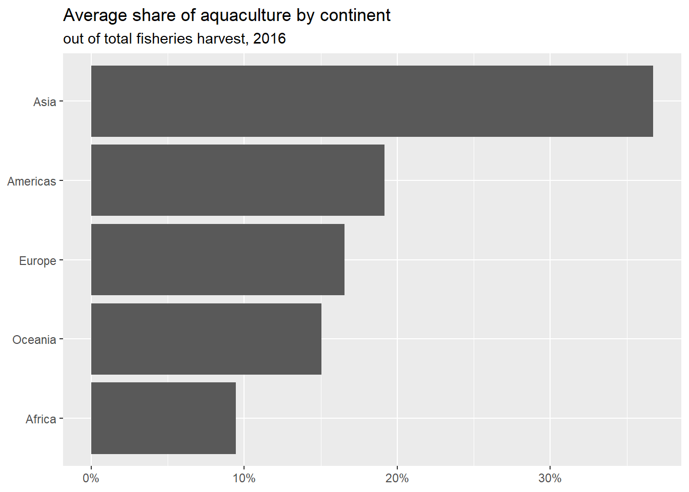
• Demo: Using your code above, create a new data frame called fisheries_summary that calculates minimum, mean, and maximum aquaculture proportion for each continent in the fisheries data.

fisheries_summary <- fisheries |> 
  group_by(continent) |>
  summarize(min_aq_prop = min(aq_prop),
            mean_aq_prop = mean(aq_prop),
            max_aq_prop = max(aq_prop))

• Demo: Then, determine which continent has the largest value of max_ap. Take the fisheries_summary data frame and order the results in descending order of max aquaculture proportion.

fisheries_summary |>
  arrange(desc(max_aq_prop))

# A tibble: 5 × 4
  continent min_aq_prop mean_aq_prop max_aq_prop
  <chr>           <dbl>        <dbl>       <dbl>
1 Africa        0             0.0943       0.803
2 Asia          0             0.367        0.782
3 Europe        0.00682       0.165        0.618
4 Americas      0             0.192        0.529
5 Oceania       0.0197        0.150        0.357

• Demo: Recreate the following plot using the data frame you have developed so far.

Hint: https://ggplot2.tidyverse.org/reference/geom_bar.html

Hint: https://forcats.tidyverse.org/reference/fct_reorder.html

Hint: We can control labels using scale_x_continious or scale_y_continous. Within this function, we can change label specifications: https://scales.r-lib.org/reference/label_percent.html

fisheries_summary |>
  ggplot(
    aes(y = fct_reorder(continent , mean_aq_prop) , x = mean_aq_prop)
  ) +
  geom_col() +
  labs(title = "Average share of aquaculture by continent",
       subtitle = "out of total fisheries harvest, 2016",
       x = NULL, 
       y = NULL) + 
  scale_x_continuous(label = label_percent(accuracy = 1))

Pivot Practice

Run the following code below. Are these data in long or wide format? Why?

x <- tibble(
  state = rep(c("MT", "NC" , "SC"),2),
  group = c(rep("C", 3), rep("D", 3)),
  obs = c(1:6)
  )

x

# A tibble: 6 × 3
  state group   obs
  <chr> <chr> <int>
1 MT    C         1
2 NC    C         2
3 SC    C         3
4 MT    D         4
5 NC    D         5
6 SC    D         6

Pivot these data so that the data are wide. i.e. Each state should be it’s own unique observation (row). Save this new data set as y.

y <- x |> 
  pivot_wider(names_from = group, values_from = obs)

Now, let’s change it back. Introducing pivot_longer. There are three things we need to consider with pivot_longer:

• What the columns will be
• names_to
• values_to

Hint: !variable.name can be read as “not this variable” or “everything but this variable”

y |>
  pivot_longer(cols = c(C,D), names_to = "group" , values_to = "obs")

# A tibble: 6 × 3
  state group   obs
  <chr> <chr> <int>
1 MT    C         1
2 MT    D         4
3 NC    C         2
4 NC    D         5
5 SC    C         3
6 SC    D         6

Pivot Practice 2

Let’s try this on a real data set.

The Portland Trailblazers are a National Basketball Association (NBA) sports team. These data reflect the points scored by 9 Portland Trailblazers players across the first 10 games of the 2021-2022 NBA season.

trailblazer <- read_csv("data/trailblazer21.csv")

Rows: 9 Columns: 11
── Column specification ────────────────────────────────────────────────────────
Delimiter: ","
chr  (1): Player
dbl (10): Game1_Home, Game2_Home, Game3_Away, Game4_Home, Game5_Home, Game6_...

ℹ Use `spec()` to retrieve the full column specification for this data.
ℹ Specify the column types or set `show_col_types = FALSE` to quiet this message.

– Take a slice at the data. Are these data in wide or long format?

slice(trailblazer)

# A tibble: 9 × 11
  Player Game1…¹ Game2…² Game3…³ Game4…⁴ Game5…⁵ Game6…⁶ Game7…⁷ Game8…⁸ Game9…⁹
  <chr>    <dbl>   <dbl>   <dbl>   <dbl>   <dbl>   <dbl>   <dbl>   <dbl>   <dbl>
1 Damia…      20      19      12      20      25      14      20      26       4
2 CJ Mc…      24      28      20      25      14      25      20      21      27
3 Norma…      14      16      NA      NA      12      14      22      23      25
4 Rober…       8       6       0       3       9       6       0       6      19
5 Jusuf…      20       9       4      17      14      13       7       6      10
6 Cody …       5       5       8      10       9       6       0       7       0
7 Anfer…      11      18      12      17       5      19      17      15      16
8 Larry…       2       8       5       8       3       8       7       0       2
9 Nassi…       7      11       5       9       8       8       4       0       7
# … with 1 more variable: Game10_Home <dbl>, and abbreviated variable names
#   ¹​Game1_Home, ²​Game2_Home, ³​Game3_Away, ⁴​Game4_Home, ⁵​Game5_Home,
#   ⁶​Game6_Away, ⁷​Game7_Away, ⁸​Game8_Away, ⁹​Game9_Home

– Pivot the data so that you have columns for Player, Game, Points. Save this as a new data set called new.blazer.

new.blazer <- trailblazer |>
  pivot_longer(cols = !Player,
               names_to = "Game", 
               values_to = "Points")

– Suppose now that you are asked to have two separate columns within these data. One column to represent Game, and one to represent Location. Make this happen below. Save your new data set as new.blazer

Hint: Run ?separate in the Console.

trailblazer |> 
  pivot_longer(cols = !Player,
               names_to = "Game",
               values_to = "Points") |>
  separate(Game, sep = "_", into = c("Game" , "Location"))

# A tibble: 90 × 4
   Player         Game   Location Points
   <chr>          <chr>  <chr>     <dbl>
 1 Damian Lillard Game1  Home         20
 2 Damian Lillard Game2  Home         19
 3 Damian Lillard Game3  Away         12
 4 Damian Lillard Game4  Home         20
 5 Damian Lillard Game5  Home         25
 6 Damian Lillard Game6  Away         14
 7 Damian Lillard Game7  Away         20
 8 Damian Lillard Game8  Away         26
 9 Damian Lillard Game9  Home          4
10 Damian Lillard Game10 Home         25
# … with 80 more rows