Regression with MLR and Logistic Regression

Packages

Note - if you don’t have the plotly or widgetframe package, you can install these before running library by writing the following code in the console:

install.packages(“plotly”) install.packages(“widgetframe”)

These packages are not necessary to finish the AE.

library(tidyverse)
library(tidymodels)
library(palmerpenguins)
library(plotly)
library(widgetframe)
library(ggridges)
library(patchwork)

Finish MLR

Last class, we fit MLR models with island and flipper length as explanatory variables vs our response body mass. Now, let’s model body mass using 2 quantitative explanatory variables to explore the difference.

Two Quantitative Explanatory Variables

How does the picture change if our two explanatory variables are quantitative?

In this example, let’s explore body mass, and it’s relationship to bill length and flipper length.

– Brainstorm, how could we visualize this?

Note: This code is beyond the scope of this course!

quanplot <- plot_ly(penguins, 
                    x = ~ flipper_length_mm, y = ~ body_mass_g, z = ~bill_length_mm,
                    marker = list(size = 3, color = "lightgray" , alpha = 0.5, 
                                  line = list(color = "gray" , width = 2))) |>
                      add_markers() |>
                      plotly::layout(scene = list(
                        xaxis = list(title = "Flipper (mm)"),
                        yaxis = list(title = "Bill (mm)"), 
                        zaxis = list(title = "Body Mass (g)")
                      )) |>
                    config(displayModeBar = FALSE)
                  frameWidget(quanplot)

Now, fit the additive model in R below:

linear_reg() |>
  set_engine("lm") |>
  fit(body_mass_g ~ flipper_length_mm + bill_length_mm, data = penguins) |>
  tidy()

# A tibble: 3 × 5
  term              estimate std.error statistic  p.value
  <chr>                <dbl>     <dbl>     <dbl>    <dbl>
1 (Intercept)       -5737.      308.      -18.6  7.80e-54
2 flipper_length_mm    48.1       2.01     23.9  7.56e-75
3 bill_length_mm        6.05      5.18      1.17 2.44e- 1

Holding bill length constant, for a 1 mm increase in flipper length, we estimate on average a 48.1 g increase in body mass

And finally, fit the interaction model in R below:

linear_reg() |>
  set_engine("lm") |>
  fit(body_mass_g ~ flipper_length_mm * bill_length_mm , data = penguins) |>
  tidy()

# A tibble: 4 × 5
  term                             estimate std.error statistic  p.value
  <chr>                               <dbl>     <dbl>     <dbl>    <dbl>
1 (Intercept)                       5091.    2925.        1.74  0.0827  
2 flipper_length_mm                   -7.31    15.0      -0.486 0.627   
3 bill_length_mm                    -229.      63.4      -3.61  0.000347
4 flipper_length_mm:bill_length_mm     1.20     0.322     3.72  0.000232

Learning goals

By the end of today, you will…

use logistic regression to fit a model for a binary response variable
fit a logistic regression model in R
think about using a logistic regression model for classification

To illustrate logistic regression, we will build a spam filter from email data. Today’s data represent incoming emails in David Diez’s (one of the authors of OpenIntro textbooks) Gmail account for the first three months of 2012 . All personally identifiable information has been removed.

email <- read_csv("data/email.csv") |>
  mutate(spam = factor(spam))

Rows: 3890 Columns: 21
── Column specification ────────────────────────────────────────────────────────
Delimiter: ","
chr   (2): winner, number
dbl  (18): spam, to_multiple, from, cc, sent_email, image, attach, dollar, i...
dttm  (1): time

ℹ Use `spec()` to retrieve the full column specification for this data.
ℹ Specify the column types or set `show_col_types = FALSE` to quiet this message.

glimpse(email)

Rows: 3,890
Columns: 21
$ spam         <fct> 0, 0, 0, 0, 0, 0, 0, 0, 0, 0, 0, 0, 0, 0, 0, 0, 0, 0, 0, …
$ to_multiple  <dbl> 0, 0, 0, 0, 0, 0, 1, 1, 0, 0, 0, 0, 0, 0, 0, 0, 0, 0, 0, …
$ from         <dbl> 1, 1, 1, 1, 1, 1, 1, 1, 1, 1, 1, 1, 1, 1, 1, 1, 1, 1, 1, …
$ cc           <dbl> 0, 0, 0, 0, 0, 0, 0, 1, 0, 0, 0, 1, 0, 1, 2, 1, 0, 2, 0, …
$ sent_email   <dbl> 0, 0, 0, 0, 0, 0, 1, 1, 0, 0, 1, 0, 0, 1, 0, 1, 0, 0, 1, …
$ time         <dttm> 2012-01-01 06:16:41, 2012-01-01 07:03:59, 2012-01-01 16:…
$ image        <dbl> 0, 0, 0, 0, 0, 0, 0, 1, 0, 0, 0, 0, 0, 0, 0, 0, 0, 0, 0, …
$ attach       <dbl> 0, 0, 0, 0, 0, 0, 0, 1, 0, 0, 0, 0, 0, 0, 0, 0, 0, 0, 0, …
$ dollar       <dbl> 0, 0, 4, 0, 0, 0, 0, 0, 0, 0, 0, 0, 0, 0, 2, 0, 5, 0, 0, …
$ winner       <chr> "no", "no", "no", "no", "no", "no", "no", "no", "no", "no…
$ inherit      <dbl> 0, 0, 1, 0, 0, 0, 0, 0, 0, 0, 0, 0, 0, 0, 0, 0, 0, 0, 0, …
$ viagra       <dbl> 0, 0, 0, 0, 0, 0, 0, 0, 0, 0, 0, 0, 0, 0, 0, 0, 0, 0, 0, …
$ password     <dbl> 0, 0, 0, 0, 2, 2, 0, 0, 0, 0, 0, 0, 0, 0, 0, 0, 1, 0, 0, …
$ num_char     <dbl> 11.370, 10.504, 7.773, 13.256, 1.231, 1.091, 4.837, 7.421…
$ line_breaks  <dbl> 202, 202, 192, 255, 29, 25, 193, 237, 69, 68, 25, 79, 191…
$ format       <dbl> 1, 1, 1, 1, 0, 0, 1, 1, 0, 1, 1, 0, 1, 1, 1, 1, 1, 1, 0, …
$ re_subj      <dbl> 0, 0, 0, 0, 0, 0, 0, 0, 0, 0, 0, 1, 0, 1, 1, 1, 0, 1, 1, …
$ exclaim_subj <dbl> 0, 0, 0, 0, 0, 0, 0, 0, 0, 0, 0, 0, 0, 0, 0, 0, 1, 0, 0, …
$ urgent_subj  <dbl> 0, 0, 0, 0, 0, 0, 0, 0, 0, 0, 0, 0, 0, 0, 0, 0, 0, 0, 0, …
$ exclaim_mess <dbl> 0, 1, 6, 48, 1, 1, 1, 18, 1, 0, 2, 1, 0, 10, 4, 10, 20, 0…
$ number       <chr> "big", "small", "small", "small", "none", "none", "big", …

The variables we’ll use in this analysis are

spam: 1 if the email is spam, 0 otherwise
exclaim_mess: The number of exclamation points in the email message

We want to use the number of exclamation points in an email to predict whether or not it is spam.

Exploratory Data Analysis

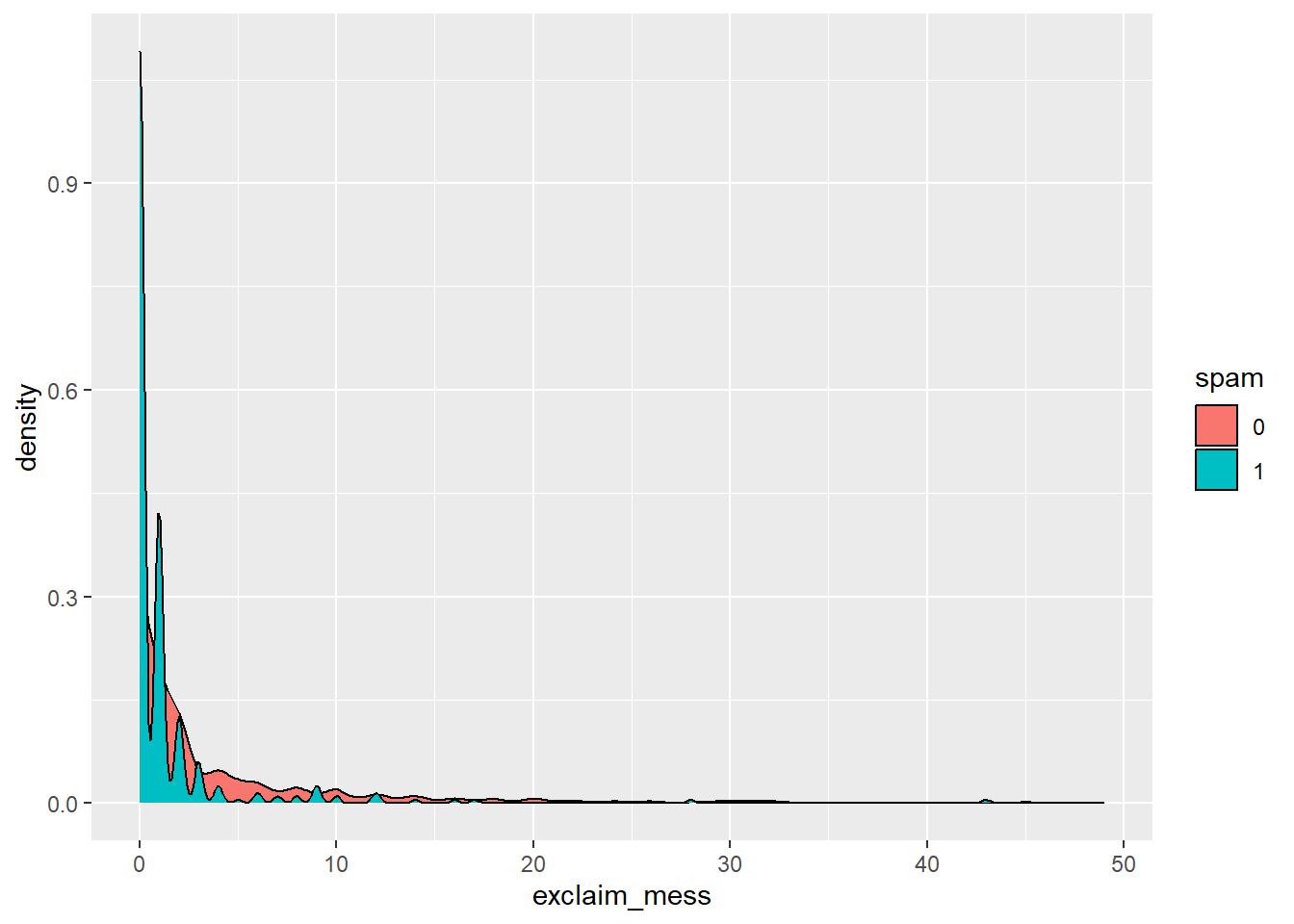
Let’s start by taking a look at our data. Create an density plot to investigate the relationship between spam and exclaim_mess. Additionally, calculate the mean number of exclamation points for both spam and non-spam emails.

email |>
  ggplot(
    aes(x = exclaim_mess , fill = spam)
  ) + 
  geom_density()

email |> 
  group_by(spam) |>
  summarize(exmean = mean(exclaim_mess))

# A tibble: 2 × 2
  spam  exmean
  <fct>  <dbl>
1 0       4.04
2 1       1.27

Let’s try a linear model (but we know it won’t work….)

Suppose we try using a linear model to describe the relationship between the number of exclamation points and whether an email is spam. Write up a linear model that models spam by exclamation marks.

linear_reg() |>
  set_engine("lm") |>
  fit(spam ~ exclaim_mess , data = email) |>
  tidy()

It won’t run!

A visualization of a linear model is below.

email |>
  ggplot() + 
  geom_jitter(aes(x = exclaim_mess, y = spam, color = spam), alpha = 0.5) + 
  geom_smooth(aes(x = exclaim_mess, y = as.numeric(spam)), method = "lm", se = FALSE, color = "black")

`geom_smooth()` using formula = 'y ~ x'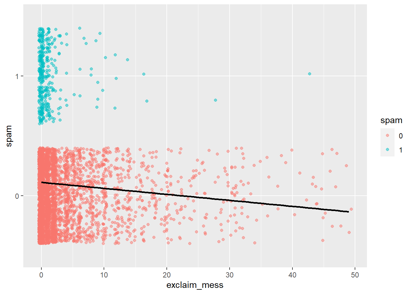

Is the linear model a good fit for the data? Why or why not?

No. That line doesn’t make sense

How do you build a model to fit a binary response variable (a categorical response variable with 2 outcomes)?

Logistic regression

Logistic regression takes in a number of explanatory variables and outputs the log-odds of “success” in a binary response variable. The log-odds are then used to predict the probability of “success”.

Let’s see what the logistic regression model looks like for our example:

Let $p$ be the probability an email is spam.

$\frac{p}{1-p}$: odds an email is spam (if p = 0.7, then the odds are 0.7/(1 - 0.7) = 2.33)
$\log\Big(\frac{p}{1-p}\Big)$: “log-odds”, i.e., the natural log, an email is spam

Then, the logistic regression model using the number of exclamation points as an explanatory variable is

\[\log\Big(\frac{p}{1-p}\Big) = \beta_0 + \beta_1 \times exclaim\_mess\]

The probability an email is spam is

\[p = \frac{\exp\{\beta_0 + \beta_1 \times exclaim\_mess\}}{1 + \exp\{\beta_0 + \beta_1 \times exclaim\_mess\}}\]

Exercise 1

Before we fit a model, we need to understand what R thinks is a success….

As a factor: ‘success’ is interpreted as:

the factor not having the first level (and hence usually of having the second level). added note: this usually means the first level alphabetically, since this is how R defines factors by default.

So, let’s assume you are in the situation where your response variable is “Yes” and “No”. The default will be to treat “No” as a failure (because alphabetical), but you can treat “No” as the success by making it the second level using fct_relevel!

As a numerical vector with values between ‘0’ and ‘1’, interpreted as the proportion of successful cases (with the total number of cases given by the ‘weights’). Or, R treats the value of 1 as a success.

Let’s fit the logistic regression model using the number of exclamation points to predict the probability an email is spam.

Things to note: We are no longer doing linear regression (we are doing logistic regression); We are not fitting a linear model (we are fitting a generalized linear model); we need to specify family = binomial in the fit function.

Name this model spam_model

spam_model <- logistic_reg() |>
  set_engine("glm") |>
  fit(spam ~ exclaim_mess , data = email, family = "binomial")

spam_model |>
  tidy()

# A tibble: 2 × 5
  term         estimate std.error statistic   p.value
  <chr>           <dbl>     <dbl>     <dbl>     <dbl>
1 (Intercept)    -1.91     0.0640    -29.8  9.82e-196
2 exclaim_mess   -0.168    0.0240     -7.02 2.21e- 12

How does the code above differ from previous code we’ve used to fit regression models?

**logistc_reg(); “glm” , family = “binomial”*

Now, compare your summary output to the estimated model below.

\[\log\Big(\frac{p}{1-p}\Big) = -1.9114 - 0.1684 \times exclaim\_mess\]

Interpretation

What does -0.1684 mean in this context?

For an additional exclaim_mess, we estimate the log odds of a spam email to decrease by 0.1684

Exercise 2

What is the probability the email is spam if it contains 10 exclamation points?

Use R as a calculator to calculate the predicted probability (do not use predict)

First, calculate the log odds by plugging in 10.

-1.91 - 0.168*10

[1] -3.59

Now, exponentiate!

exp(-3.59) / (1+exp(-3.59))

[1] 0.02685712

The predicted probability of a spam email when the number of exclamation points equals 10 is 0.027

We can use the predict function in R to produce the probability as well.

Note, in logistic, we have to pull out the model estimates using $fit. The type=“response” option tells R to output probabilities of the form P(Y = 1|X), as opposed to other information such as the logit.

new_email <- tibble(exclaim_mess = 2)

predict(spam_model$fit, new_email) # log-odds

        1 
-2.248108

round(predict(spam_model$fit, new_email, type = "response"),3) # probability

    1 
0.096

Exercise 3 - Classification

We have the probability an email is spam, but ultimately we want to use the probability to classify an email as spam or not spam. Therefore, we need to set a decision-making threshold, such that an email is classified as spam if the predicted probability is greater than the threshold and not spam otherwise.

Suppose you are a data scientist working on a spam filter. You must determine how high the predicted probability must be before you think it would be reasonable to call it spam and put it in the junk folder (which the user is unlikely to check).

What are some tradeoffs you would consider as you set the decision-making threshold? Discuss with your neighbor.

AWV: Think about benefits and consequences of making a threshold to low vs to high in this context…. what about in a situation more serious?

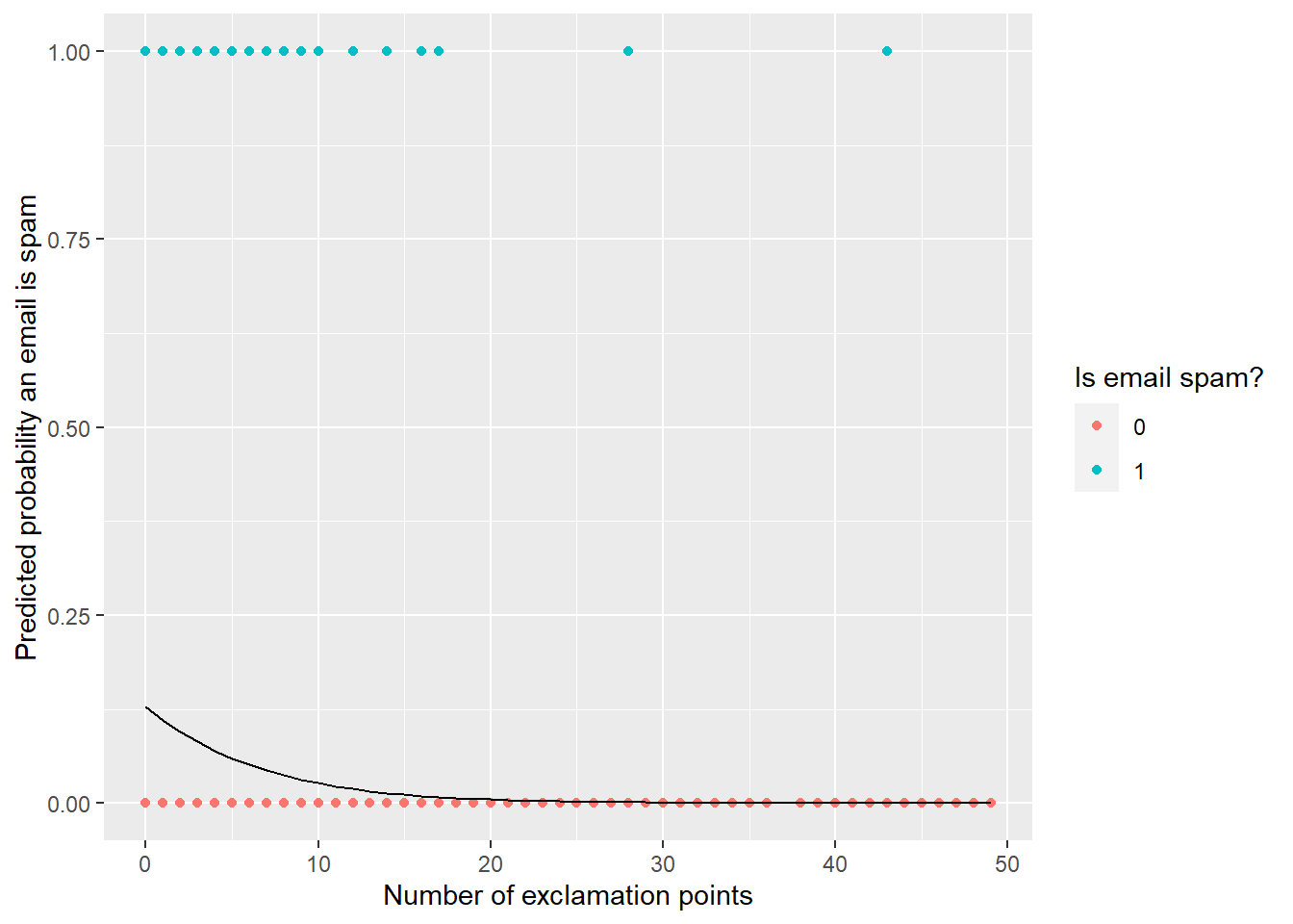
email <- email |>
  mutate(pred_prob = predict(spam_model$fit, type = "response"))
ggplot(data = email) + 
  geom_point(aes(x = exclaim_mess, y = as.numeric(spam) -1, 
                        color = spam)) + 
  geom_line(aes(x = exclaim_mess, y = pred_prob)) + 
  labs(x = "Number of exclamation points", 
       y = "Predicted probability an email is spam", 
       color = "Is email spam?"
       )

Next time, we will discuss how to evaluate these models with testing + training data sets!