MLR - Logistic Regression

Day 10

Dr. Elijah Meyer

Duke University
STA 199 - Summer 2023

June 8th

Checklist

– Clone ae-10

– Homework 3 Due Tuesday (6-13)

– Project Proposal due Monday (6-12)

— Turn in on GitHub

— Lab today is a project work day

Warm Up: Question 1

– What is the main difference between Simple Linear Regression and Multiple Linear Regression?

Warm Up: Question 2

– What is the main difference between an additive model and an interaction model?

Goals

– Understand R-squared vs Adjusted R-squared

– What, why and how of logistic regression

More about R-Squared vs Adjusted R-Squared

R-squared has…

  • A meaningful definition

  • a relationship with cor when in the SLR case

R-Squared

R-squared

More about R-Squared vs Adjusted R-Squared

When can we use R-squared for model selection?

  • When models have the same number of variables

  • Why can’t we use it to compare models with different number of variables? See ae-09 for demonstration.

R-squared: Takeaway

– statistical measure in a regression model that determines the proportion of variance in the response variable that can be explained by the explanatory variable(s).

– The more variables you include, the larger the R-squared value will be (always)

More about R-Squared vs Adjusted R-Squared

Adjusted R-squared …

  • Doesn’t have a clean definition

  • Is very useful for model selection

Adjusted R-Squared

Takeaway: Adds a penalty for “unimportant” predictors (x’s)

Any questions?

Finish MLR

– clone ae-10

– finish MLR (2 quantitative explanatory variables)

Logistic Regression

Goals

– The What, Why, and How of Logistic Regression

What is Logistic Regreesion

  • Similar to linear regression…. but

  • Modeling tool when our response is categorical

What we will do today

– This type of model is called a generalized linear model

Start from the beginning

Terms

– Bernoulli Distribution

  • 2 outcomes: Success (p) or Failure (1-p)

  • \(y_i\) ~ Bern(p)

  • What we can do is we can use our explanatory variable(s) to model p

2 Steps

– 1: Define a linear model

– 2: Define a link function

A linear model

\(\eta_i = \beta_o + \beta_1*X_i + ...\)

Note: \(\eta_i\) is some response of our linear model

  • But we can’t stop here… \(\eta_i\) isn’t the probability of success of our response

  • Think about what a linear model looks like

Next steps

– Preform a transformation to our response variable so it has the appropriate range of values

– “Link” our linear model to the paramater of the outcome distribution

\(y_i\) ~ Bern(p)

Generalized linear model

  • Next, we need a link function that relates the linear model to the parameter of the outcome distribution i.e. transform the linear model to have an appropriate range
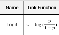
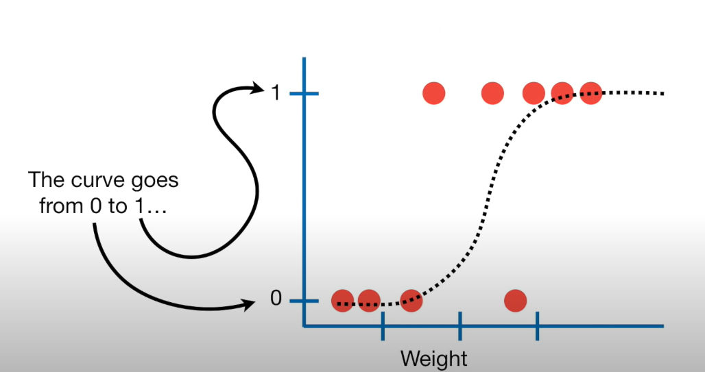
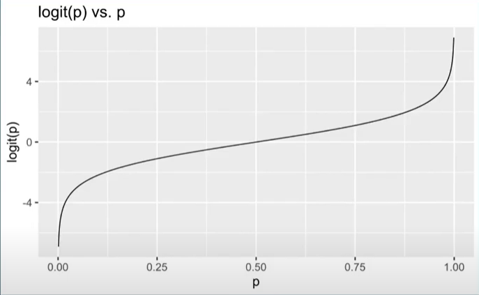
What’s this look like

Takes a [0,1] probability and maps it to log odds (-\(\infty\) to \(\infty\).)

Almost….

This isn’t exactly what we need though…..

Will help us get to our goal

So we have a generalized linear model (GLM)

  • \(logit(p_i)\) = \(\widehat{\beta_o} +\widehat{\beta}_1X1_i + ....\)

  • logit(p) is also known as the log-odds

  • logit(p) = \(log(\frac{p}{1-p})\)

  • \(log(\frac{p}{1-p})\) = \(\widehat{\beta_o} +\widehat{\beta}_1X1 + ....\)
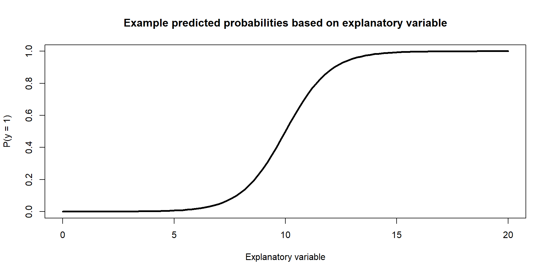
One final fix

– Recall, the goal is to take values between -\(\infty\) and \(\infty\) and map them to probabilities. We need the opposite of the link function… or the inverse

– How do we take the inverse of a natural log?

  • Taking the inverse of the logit function will map arbitrary real values back to the range [0, 1]

So

We need to take the inverse of the logit function

  • \[log(\frac{p}{1-p}) = \widehat{\beta_o} +\widehat{\beta}_1X1 + ....\]

Math Time

What we will do today

Calculate probabilities of success of a response based on values of explanatory variable x.